A Short Introduction to the blorr Package
Aravind Hebbali
Source:vignettes/introduction.Rmd
introduction.RmdIntroduction
The blorr package offers tools for building and validating binary
logistic regression models. It is most suitable for
beginner/intermediate R users and those who teach statistics using R.
The API is very simple and most of the functions take either a
data.frame/tibble or a model as
input. blorr use consistent prefix
blr_ for easy tab completion.
Installation
You can install blorr using:
install.packages("blorr")The documentation of the package can be found at https://blorr.rsquaredacademy.com. This vignette gives a quick tour of the package.
Data
To demonstrate the features of blorr, we will use the bank marketing data set. The data is related with direct marketing campaigns of a Portuguese banking institution. The marketing campaigns were based on phone calls. Often, more than one contact to the same client was required, in order to access if the product (bank term deposit) would be (‘yes’) or not (‘no’) subscribed. It contains a random sample (~4k) of the original data set which can be found at https://archive.ics.uci.edu/ml/datasets/bank+marketing.
Bivariate Analysis
Let us begin with careful bivariate analysis of each possible variable and the outcome variable. We will use information value and likelihood ratio chi square test for selecting the initial set of predictors for our model. The bivariate analysis is currently avialable for categorical predictors only.
blr_bivariate_analysis(bank_marketing, y, job, marital, education, default,
  housing, loan, contact, poutcome)
#>                           Bivariate Analysis
#> ----------------------------------------------------------------------
#> Variable     Information Value    LR Chi Square    LR DF    LR p-value
#> ----------------------------------------------------------------------
#>    job             0.16              75.2690        11        0.0000
#>  marital           0.05              21.6821         2        0.0000
#> education          0.05              25.0466         3        0.0000
#>  default           0.02              6.0405          1        0.0140
#>  housing           0.16              72.2813         1        0.0000
#>   loan             0.06              26.6615         1        0.0000
#>  contact           0.31             124.3834         2        0.0000
#> poutcome           0.53             270.6450         3        0.0000
#> ----------------------------------------------------------------------
Weight of Evidence & Information Value
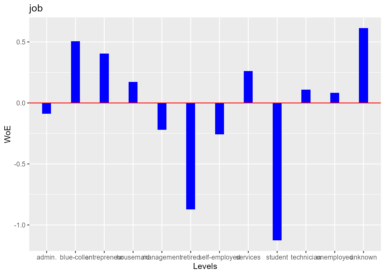
Weight of evidence (WoE) is used to assess the relative risk of di¤erent attributes for a characteristic and as a means to transform characteristics into variables. It is also a very useful tool for binning. The WoE for any group with average odds is zero. A negative WoE indicates that the proportion of defaults is higher for that attribute than the overall proportion and indicates higher risk.
The information value is used to rank order variables in terms of their predictive power. A high information value indicates a high ability to discriminate. Values for the information value will always be positive and may be above 3 when assessing highly predictive characteristics. Characteristics with information values less than 0:10 are typically viewed as weak, while values over 0.30 are sought after.
blr_woe_iv(bank_marketing, job, y)
#>                                Weight of Evidence
#> --------------------------------------------------------------------------------
#>    levels        count_0s    count_1s    dist_0s    dist_1s        woe      iv
#> --------------------------------------------------------------------------------
#>  management        809         130          0.20       0.25      -0.22     0.01
#>  technician        682          79          0.17       0.15       0.11     0.00
#> entrepreneur       139          12          0.03       0.02       0.40     0.00
#>  blue-collar       937          73          0.23       0.14       0.51     0.05
#>    unknown          29          2           0.01       0.00       0.61     0.00
#>    retired         152          47          0.04       0.09      -0.87     0.05
#>    admin.          433          61          0.11       0.12      -0.09     0.00
#>   services         392          39          0.10       0.08       0.26     0.01
#> self-employed      132          22          0.03       0.04      -0.26     0.00
#>  unemployed        126          15          0.03       0.03       0.08     0.00
#>   housemaid        110          12          0.03       0.02       0.17     0.00
#>    student          63          25          0.02       0.05      -1.13     0.04
#> --------------------------------------------------------------------------------
#>
#>       Information Value
#> -----------------------------
#> Variable    Information Value
#> -----------------------------
#>   job            0.1594
#> -----------------------------
Multiple Variables
We can generate the weight of evidence and information value for
multiple variables using blr_woe_iv_stats().
blr_woe_iv_stats(bank_marketing, y, job, marital, education)
#> Variable: job
#>
#>                                Weight of Evidence
#> --------------------------------------------------------------------------------
#>    levels        count_0s    count_1s    dist_0s    dist_1s        woe      iv
#> --------------------------------------------------------------------------------
#>  management        809         130          0.20       0.25      -0.22     0.01
#>  technician        682          79          0.17       0.15       0.11     0.00
#> entrepreneur       139          12          0.03       0.02       0.40     0.00
#>  blue-collar       937          73          0.23       0.14       0.51     0.05
#>    unknown          29          2           0.01       0.00       0.61     0.00
#>    retired         152          47          0.04       0.09      -0.87     0.05
#>    admin.          433          61          0.11       0.12      -0.09     0.00
#>   services         392          39          0.10       0.08       0.26     0.01
#> self-employed      132          22          0.03       0.04      -0.26     0.00
#>  unemployed        126          15          0.03       0.03       0.08     0.00
#>   housemaid        110          12          0.03       0.02       0.17     0.00
#>    student          63          25          0.02       0.05      -1.13     0.04
#> --------------------------------------------------------------------------------
#>
#>       Information Value
#> -----------------------------
#> Variable    Information Value
#> -----------------------------
#>   job            0.1594
#> -----------------------------
#>
#>
#> Variable: marital
#>
#>                             Weight of Evidence
#> ---------------------------------------------------------------------------
#>  levels     count_0s    count_1s    dist_0s    dist_1s        woe      iv
#> ---------------------------------------------------------------------------
#> married       2467        273          0.62       0.53       0.15     0.01
#>  single       1079        191          0.27       0.37      -0.32     0.03
#> divorced      458          53          0.11       0.10       0.11     0.00
#> ---------------------------------------------------------------------------
#>
#>       Information Value
#> -----------------------------
#> Variable    Information Value
#> -----------------------------
#> marital          0.0464
#> -----------------------------
#>
#>
#> Variable: education
#>
#>                              Weight of Evidence
#> ----------------------------------------------------------------------------
#>  levels      count_0s    count_1s    dist_0s    dist_1s        woe      iv
#> ----------------------------------------------------------------------------
#> tertiary       1104        195          0.28       0.38      -0.31     0.03
#> secondary      2121        231          0.53       0.45       0.17     0.01
#>  unknown       154          25          0.04       0.05      -0.23     0.00
#>  primary       625          66          0.16       0.13       0.20     0.01
#> ----------------------------------------------------------------------------
#>
#>       Information Value
#> ------------------------------
#> Variable     Information Value
#> ------------------------------
#> education         0.0539
#> ------------------------------
blr_woe_iv() and blr_woe_iv_stats() are
currently avialable for categorical predictors only.
Stepwise Selection
For the initial/ first cut model, all the independent variables are
put into the model. Our goal is to include a limited number of
independent variables (5-15) which are all significant, without
sacrificing too much on the model performance. The rationale behind
not-including too many variables is that the model would be over fitted
and would become unstable when tested on the validation sample. The
variable reduction is done using forward or backward or stepwise
variable selection procedures. We will use
blr_step_aic_both() to shortlist predictors for our
model.
Model
Selection Summary
blr_step_aic_both(model)
#> Stepwise Selection Method
#> -------------------------
#>
#> Candidate Terms:
#>
#> 1 . age
#> 2 . job
#> 3 . marital
#> 4 . education
#> 5 . default
#> 6 . balance
#> 7 . housing
#> 8 . loan
#> 9 . contact
#> 10 . day
#> 11 . month
#> 12 . duration
#> 13 . campaign
#> 14 . pdays
#> 15 . previous
#> 16 . poutcome
#>
#>
#> Variables Entered/Removed:
#>
#> - duration added
#> - poutcome added
#> - month added
#> - contact added
#> - housing added
#> - loan added
#> - campaign added
#> - marital added
#> - education added
#> - age added
#>
#> No more variables to be added or removed.
#>
#>
#>                      Stepwise Summary
#> ---------------------------------------------------------
#> Variable      Method       AIC         BIC       Deviance
#> ---------------------------------------------------------
#> duration     addition    2674.384    2687.217    2670.384
#> poutcome     addition    2396.014    2428.097    2386.014
#> month        addition    2274.109    2376.773    2242.109
#> contact      addition    2207.884    2323.381    2171.884
#> housing      addition    2184.550    2306.463    2146.550
#> loan         addition    2171.972    2300.302    2131.972
#> campaign     addition    2164.164    2298.910    2122.164
#> marital      addition    2158.524    2306.103    2112.524
#> education    addition    2155.837    2322.666    2103.837
#> age          addition    2154.272    2327.517    2100.272
#> ---------------------------------------------------------
Plot
model %>%
  blr_step_aic_both() %>%
  plot()
#> Stepwise Selection Method
#> -------------------------
#>
#> Candidate Terms:
#>
#> 1 . age
#> 2 . job
#> 3 . marital
#> 4 . education
#> 5 . default
#> 6 . balance
#> 7 . housing
#> 8 . loan
#> 9 . contact
#> 10 . day
#> 11 . month
#> 12 . duration
#> 13 . campaign
#> 14 . pdays
#> 15 . previous
#> 16 . poutcome
#>
#>
#> Variables Entered/Removed:
#>
#> - duration added
#> - poutcome added
#> - month added
#> - contact added
#> - housing added
#> - loan added
#> - campaign added
#> - marital added
#> - education added
#> - age added
#>
#> No more variables to be added or removed.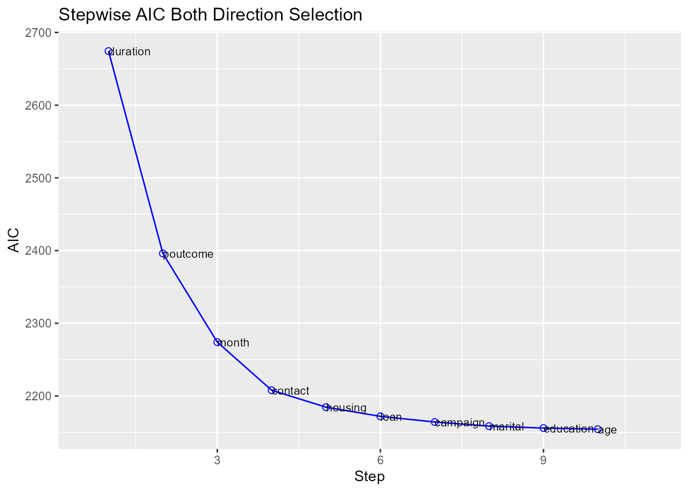
Regression Output
Model
We can use bivariate analysis and stepwise selection procedure to
shortlist predictors and build the model using the glm().
The predictors used in the below model are for illustration purposes and
not necessarily shortlisted from the bivariate analysis and variable
selection procedures.
model <- glm(y ~  age + duration + previous + housing + default +
             loan + poutcome + job + marital, data = bank_marketing,
             family = binomial(link = 'logit'))
Use blr_regress() to generate comprehensive regression
output. It accepts either of the following
- model built using
glm() - model formula and data
Using Model
Let us look at the output generated from
blr_regress():
blr_regress(model)
#>                              Model Overview
#> ------------------------------------------------------------------------
#> Data Set    Resp Var    Obs.    Df. Model    Df. Residual    Convergence
#> ------------------------------------------------------------------------
#>   data         y        4521      4520           4498           TRUE
#> ------------------------------------------------------------------------
#>
#>                     Response Summary
#> --------------------------------------------------------
#> Outcome        Frequency        Outcome        Frequency
#> --------------------------------------------------------
#>    0             4004              1              517
#> --------------------------------------------------------
#>
#>                      Maximum Likelihood Estimates
#> -----------------------------------------------------------------------
#>    Parameter        DF    Estimate    Std. Error    z value     Pr(>|z|)
#> -----------------------------------------------------------------------
#>   (Intercept)       1     -5.1347        0.3728    -13.7729      0.0000
#>       age           1      0.0096        0.0067      1.4299      0.1528
#>     duration        1      0.0042         2e-04     20.7853      0.0000
#>     previous        1     -0.0357        0.0392     -0.9089      0.3634
#>    housingno        1      0.7894        0.1232      6.4098      0.0000
#>    defaultyes       1     -0.8691        0.6919     -1.2562      0.2091
#>      loanno         1      0.6598        0.1945      3.3925       7e-04
#> poutcomefailure     1      0.6085        0.2012      3.0248      0.0025
#>  poutcomeother      1      1.1354        0.2700      4.2057      0.0000
#> poutcomesuccess     1      3.2481        0.2462     13.1913      0.0000
#>  jobtechnician      1     -0.2713        0.1806     -1.5019      0.1331
#> jobentrepreneur     1     -0.7041        0.3809     -1.8486      0.0645
#>  jobblue-collar     1     -0.6132        0.1867     -3.2851      0.0010
#>    jobunknown       1     -0.9932        0.8226     -1.2073      0.2273
#>    jobretired       1      0.3197        0.2729      1.1713      0.2415
#>    jobadmin.        1      0.1120        0.2001      0.5599      0.5755
#>   jobservices       1     -0.1750        0.2265     -0.7728      0.4397
#> jobself-employed    1     -0.1408        0.3009     -0.4680      0.6398
#>  jobunemployed      1     -0.6581        0.3432     -1.9174      0.0552
#>   jobhousemaid      1     -0.7456        0.3932     -1.8963      0.0579
#>    jobstudent       1      0.1927        0.3433      0.5613      0.5746
#>  maritalsingle      1      0.5451        0.1387      3.9299       1e-04
#> maritaldivorced     1     -0.1989        0.1986     -1.0012      0.3167
#> -----------------------------------------------------------------------
#>
#>  Association of Predicted Probabilities and Observed Responses
#> ---------------------------------------------------------------
#> % Concordant          0.8886          Somers' D        0.7773
#> % Discordant          0.1114          Gamma            0.7773
#> % Tied                0.0000          Tau-a            0.1575
#> Pairs                2070068          c                0.8886
#> ---------------------------------------------------------------
If you want to examine the odds ratio estimates, set
odd_conf_limit to TRUE. The odds ratio
estimates are not explicitly computed as we observed considerable
increase in computation time when dealing with large data sets.
Using Formula
Let us use the model formula and the data set to generate the above results.
blr_regress(y ~  age + duration + previous + housing + default +
             loan + poutcome + job + marital, data = bank_marketing)
#>                              Model Overview
#> ------------------------------------------------------------------------
#> Data Set    Resp Var    Obs.    Df. Model    Df. Residual    Convergence
#> ------------------------------------------------------------------------
#>   data         y        4521      4520           4498           TRUE
#> ------------------------------------------------------------------------
#>
#>                     Response Summary
#> --------------------------------------------------------
#> Outcome        Frequency        Outcome        Frequency
#> --------------------------------------------------------
#>    0             4004              1              517
#> --------------------------------------------------------
#>
#>                      Maximum Likelihood Estimates
#> -----------------------------------------------------------------------
#>    Parameter        DF    Estimate    Std. Error    z value     Pr(>|z|)
#> -----------------------------------------------------------------------
#>   (Intercept)       1     -5.1347        0.3728    -13.7729      0.0000
#>       age           1      0.0096        0.0067      1.4299      0.1528
#>     duration        1      0.0042         2e-04     20.7853      0.0000
#>     previous        1     -0.0357        0.0392     -0.9089      0.3634
#>    housingno        1      0.7894        0.1232      6.4098      0.0000
#>    defaultyes       1     -0.8691        0.6919     -1.2562      0.2091
#>      loanno         1      0.6598        0.1945      3.3925       7e-04
#> poutcomefailure     1      0.6085        0.2012      3.0248      0.0025
#>  poutcomeother      1      1.1354        0.2700      4.2057      0.0000
#> poutcomesuccess     1      3.2481        0.2462     13.1913      0.0000
#>  jobtechnician      1     -0.2713        0.1806     -1.5019      0.1331
#> jobentrepreneur     1     -0.7041        0.3809     -1.8486      0.0645
#>  jobblue-collar     1     -0.6132        0.1867     -3.2851      0.0010
#>    jobunknown       1     -0.9932        0.8226     -1.2073      0.2273
#>    jobretired       1      0.3197        0.2729      1.1713      0.2415
#>    jobadmin.        1      0.1120        0.2001      0.5599      0.5755
#>   jobservices       1     -0.1750        0.2265     -0.7728      0.4397
#> jobself-employed    1     -0.1408        0.3009     -0.4680      0.6398
#>  jobunemployed      1     -0.6581        0.3432     -1.9174      0.0552
#>   jobhousemaid      1     -0.7456        0.3932     -1.8963      0.0579
#>    jobstudent       1      0.1927        0.3433      0.5613      0.5746
#>  maritalsingle      1      0.5451        0.1387      3.9299       1e-04
#> maritaldivorced     1     -0.1989        0.1986     -1.0012      0.3167
#> -----------------------------------------------------------------------
#>
#>  Association of Predicted Probabilities and Observed Responses
#> ---------------------------------------------------------------
#> % Concordant          0.8886          Somers' D        0.7773
#> % Discordant          0.1114          Gamma            0.7773
#> % Tied                0.0000          Tau-a            0.1575
#> Pairs                2070068          c                0.8886
#> ---------------------------------------------------------------
Model Fit Statistics
Model fit statistics are available to assess how well the model fits the data and to compare two different models.The output includes likelihood ratio test, AIC, BIC and a host of pseudo r-squared measures. You can read more about pseudo r-squared here.
Single Model
blr_model_fit_stats(model)
#>                                Model Fit Statistics
#> ----------------------------------------------------------------------------------
#> Log-Lik Intercept Only:     -1607.330    Log-Lik Full Model:             -1123.340
#> Deviance(4498):              2246.679    LR(22):                           967.980
#>                                          Prob > LR:                          0.000
#> MCFadden's R2                   0.301    McFadden's Adj R2:                  0.287
#> ML (Cox-Snell) R2:              0.193    Cragg-Uhler(Nagelkerke) R2:         0.379
#> McKelvey & Zavoina's R2:        0.388    Efron's R2:                         0.278
#> Count R2:                       0.904    Adj Count R2:                       0.157
#> BIC:                         2440.259    AIC:                             2292.679
#> ----------------------------------------------------------------------------------
Model Validation
Confusion Matrix
In the event of deciding a cut-off point on the probability scores of a logistic regression model, a confusion matrix is created corresponding to a particular cut-off. The observations with probability scores above the cut-off score are predicted to be events and those below the cut-off score, as non-events. The confusion matrix, a 2X2 table, then calculates the number of correctly classified and miss-classified observations.
blr_confusion_matrix(model, cutoff = 0.5)
#> Confusion Matrix and Statistics
#>
#>           Reference
#> Prediction    0    1
#>          0 3920  352
#>          1   84  165
#>
#>
#>                 Accuracy : 0.9036
#>      No Information Rate : 0.8856
#>
#>                    Kappa : 0.3851
#>
#> McNemars's Test P-Value  : 0.0000
#>
#>              Sensitivity : 0.3191
#>              Specificity : 0.9790
#>           Pos Pred Value : 0.6627
#>           Neg Pred Value : 0.9176
#>               Prevalence : 0.1144
#>           Detection Rate : 0.0365
#>     Detection Prevalence : 0.0551
#>        Balanced Accuracy : 0.6491
#>                Precision : 0.6627
#>                   Recall : 0.3191
#>
#>         'Positive' Class : 1
The validity of a cut-off is measured using sensitivity, specificity and accuracy.
Sensitivity: The % of correctly classified events out of all events = TP / (TP + FN)
Specificity: The % of correctly classified non-events out of all non-events = TN / (TN + FP)
Accuracy: The % of correctly classified observation over all observations = (TP + TN) / (TP + FP + TN + FN)
True Positive (TP) : Events correctly classified as events.
True Negative (TN) : Non-Events correctly classified as non-events.
False Positive (FP): Non-events miss-classified as events.
False Negative (FN): Events miss-classified as non-events.
For a standard logistic model, the higher is the cut-off, the lower will be the sensitivity and the higher would be the specificity. As the cut-off is decreased, sensitivity will go up, as then more events would be captured. Also, specificity will go down, as more non-events would miss-classified as events. Hence a trade-off is done based on the requirements. For example, if we are looking to capture as many events as possible, and we can afford to have miss-classified non-events, then a low cut-off is taken.
Hosmer Lemeshow Test
Hosmer and Lemeshow developed a goodness-of-fit test for logistic regression models with binary responses. The test involves dividing the data into approximately ten groups of roughly equal size based on the percentiles of the estimated probabilities. The observations are sorted in increasing order of their estimated probability of having an even outcome. The discrepancies between the observed and expected number of observations in these groups are summarized by the Pearson chi-square statistic, which is then compared to chi-square distribution with t degrees of freedom, where t is the number of groups minus 2. Lower values of Goodness-of-fit are preferred.
blr_test_hosmer_lemeshow(model)
#>            Partition for the Hosmer & Lemeshow Test
#> --------------------------------------------------------------
#>                         def = 1                 def = 0
#> Group    Total    Observed    Expected    Observed    Expected
#> --------------------------------------------------------------
#>   1       453        2          5.14        451        447.86
#>   2       452        3          8.63        449        443.37
#>   3       452        4         11.88        448        440.12
#>   4       452        7         15.29        445        436.71
#>   5       452        14        19.39        438        432.61
#>   6       452        10        24.97        442        427.03
#>   7       452        31        33.65        421        418.35
#>   8       452        62        49.74        390        402.26
#>   9       452       128        88.10        324        363.90
#>  10       452       256        260.21       196        191.79
#> --------------------------------------------------------------
#>
#>      Goodness of Fit Test
#> ------------------------------
#> Chi-Square    DF    Pr > ChiSq
#> ------------------------------
#>  52.9942      8       0.0000
#> ------------------------------
Gains Table & Lift Chart
A lift curve is a graphical representation of the % of cumulative events captured at a specific cut-off. The cut-off can be a particular decile or a percentile. Similar, to rank ordering procedure, the data is in descending order of the scores and is then grouped into deciles/percentiles. The cumulative number of observations and events are then computed for each decile/percentile. The lift curve is the created using the cumulative % population as the x-axis and the cumulative percentage of events as the y-axis.
blr_gains_table(model)
#>    decile total   1   0       ks  tp   tn   fp  fn sensitivity specificity
#> 1       1   452 256 196 44.62134 256 3808  196 261    49.51644    95.10490
#> 2       2   452 128 324 61.28765 384 3484  520 133    74.27466    87.01299
#> 3       3   452  62 390 63.53965 446 3094  910  71    86.26692    77.27273
#> 4       4   452  31 421 59.02130 477 2673 1331  40    92.26306    66.75824
#> 5       5   452  10 442 49.91657 487 2231 1773  30    94.19729    55.71928
#> 6       6   452  14 438 41.68544 501 1793 2211  16    96.90522    44.78022
#> 7       7   452   7 445 31.92552 508 1348 2656   9    98.25919    33.66633
#> 8       8   452   4 448 21.51040 512  900 3104   5    99.03288    22.47752
#> 9       9   452   3 449 10.87689 515  451 3553   2    99.61315    11.26374
#> 10     10   453   2 451  0.00000 517    0 4004   0   100.00000     0.00000
#>    accuracy
#> 1  89.89162
#> 2  85.55629
#> 3  78.30126
#> 4  69.67485
#> 5  60.11944
#> 6  50.74099
#> 7  41.05286
#> 8  31.23203
#> 9  21.36695
#> 10 11.43552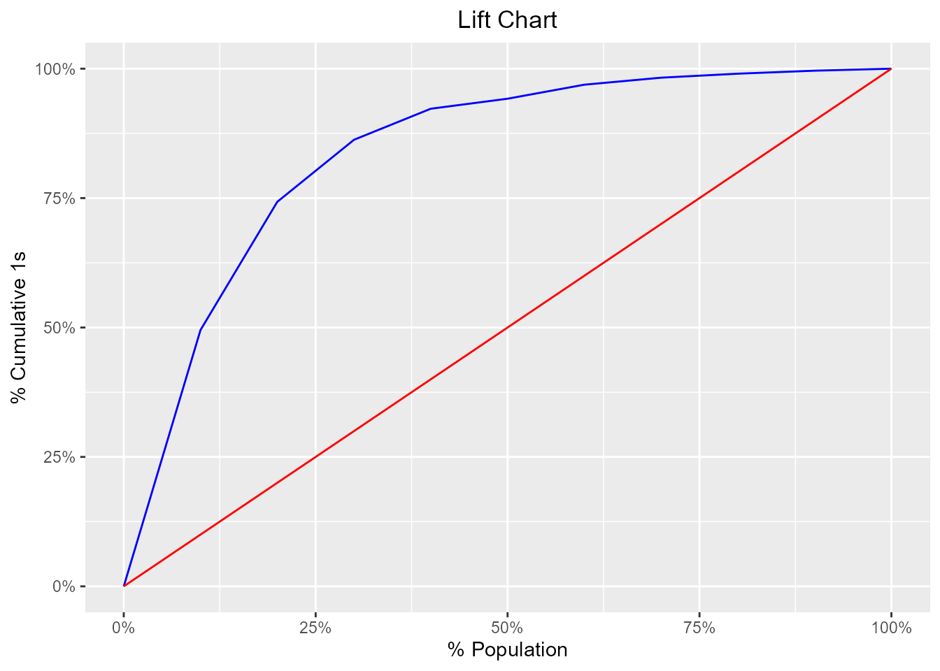
ROC Curve
ROC curve is a graphical representation of the validity of cut-offs for a logistic regression model. The ROC curve is plotted using the sensitivity and specificity for all possible cut-offs, i.e., all the probability scores. The graph is plotted using sensitivity on the y-axis and 1-specificity on the x-axis. Any point on the ROC curve represents a sensitivity X (1-specificity) measure corresponding to a cut-off. The area under the ROC curve is used as a validation measure for the model – the bigger the area the better is the model.
model %>%
    blr_gains_table() %>%
  blr_roc_curve()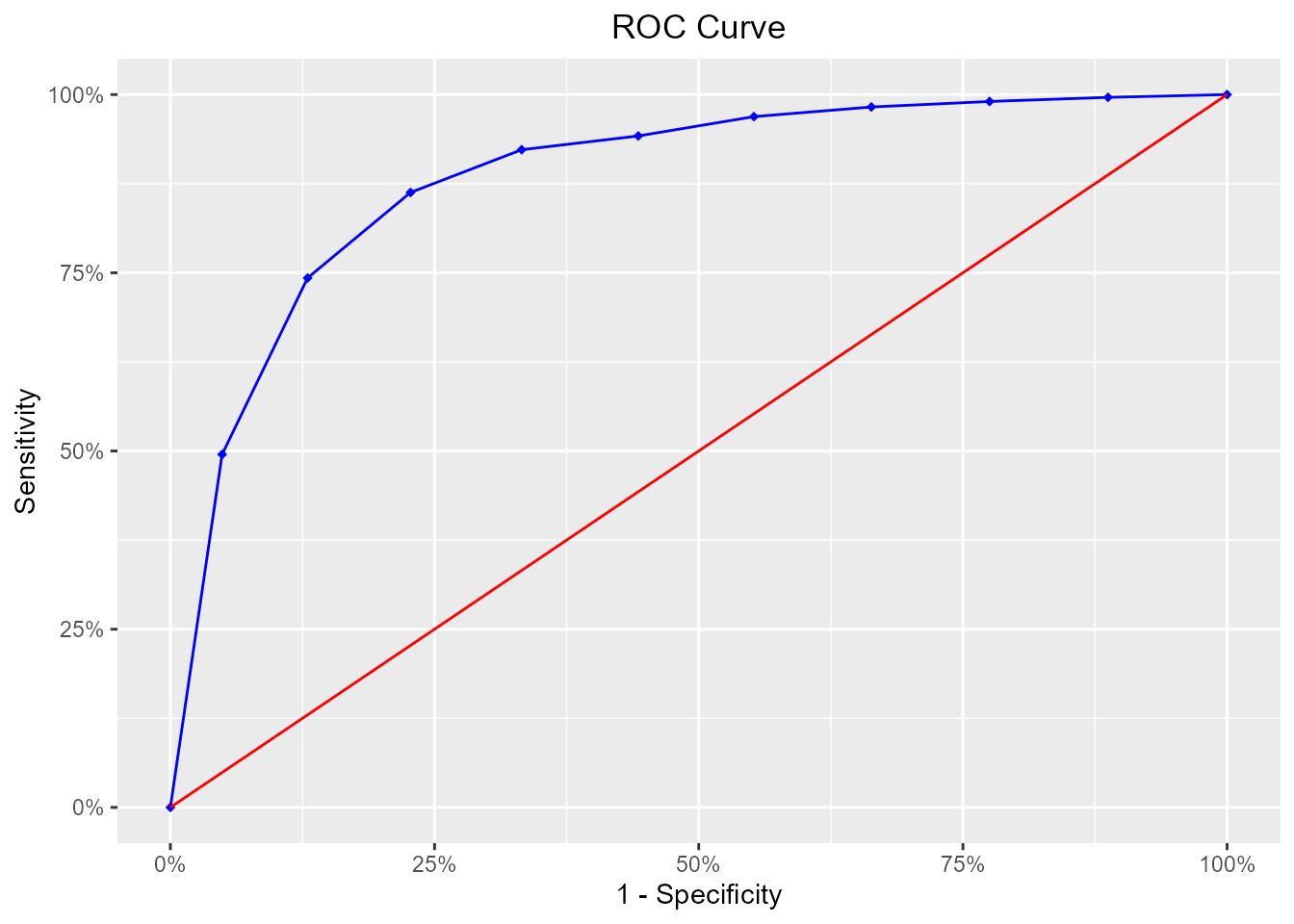
KS Chart
The KS Statistic is again a measure of model efficiency, and it is created using the lift curve. The lift curve is created to plot % events. If we also plot % non-events on the same scale, with % population at x-axis, we would get another curve. The maximum distance between the lift curve for events and that for non-events is termed as KS. For a good model, KS should be big (>=0.3) and should occur as close to the event rate as possible.
model %>%
    blr_gains_table() %>%
  blr_ks_chart()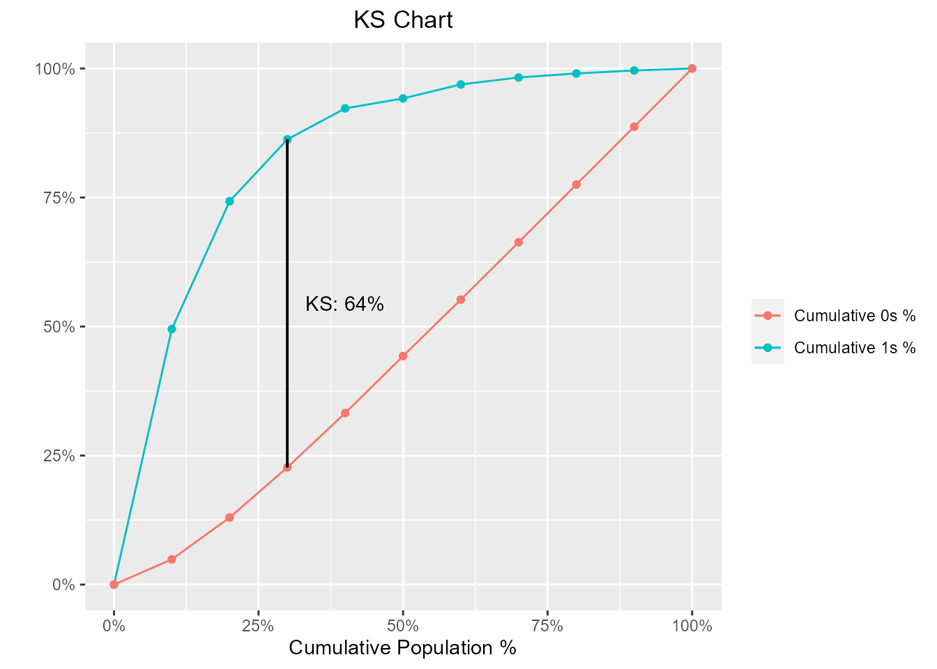
Decile Lift Chart
The decile lift chart displays the lift over the global mean event rate for each decile. For a model with good discriminatory power, the top deciles should have an event/conversion rate greater than the global mean.
model %>%
  blr_gains_table() %>%
  blr_decile_lift_chart()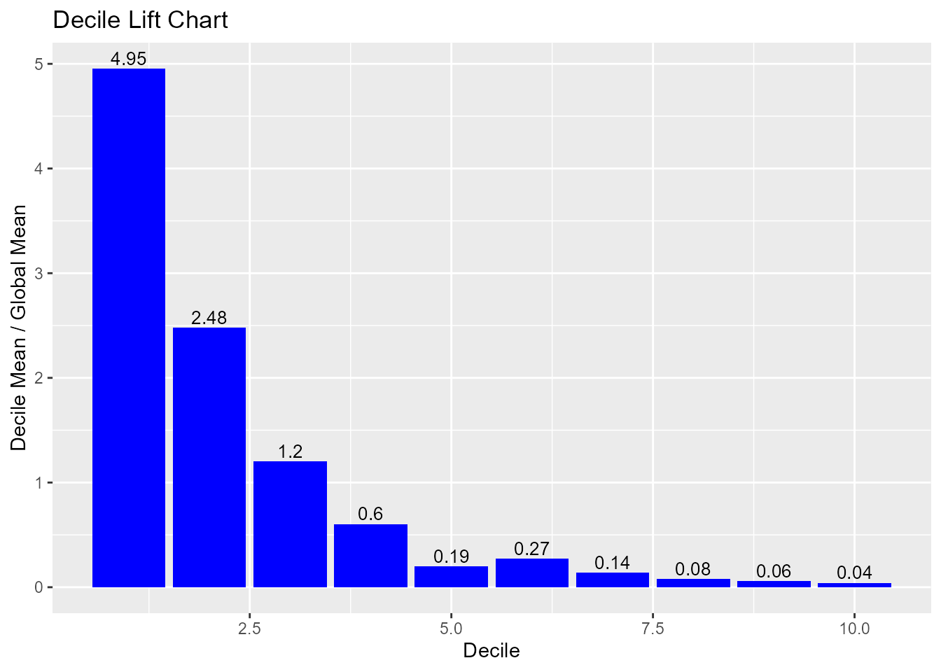
Capture Rate by Decile
If the model has good discriminatory power, the top deciles should have a higher event/conversion rate compared to the bottom deciles.
model %>%
  blr_gains_table() %>%
  blr_decile_capture_rate()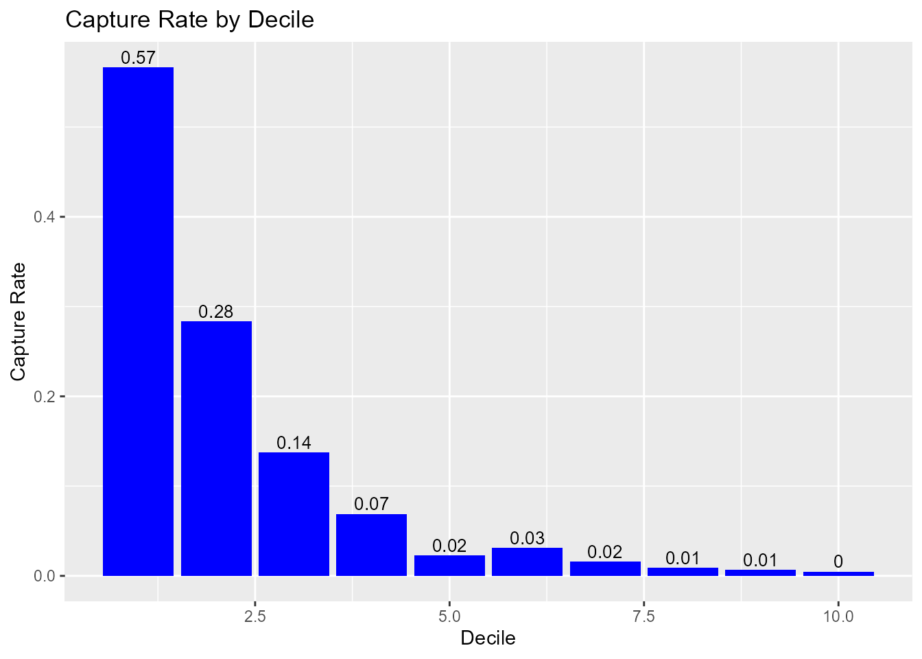
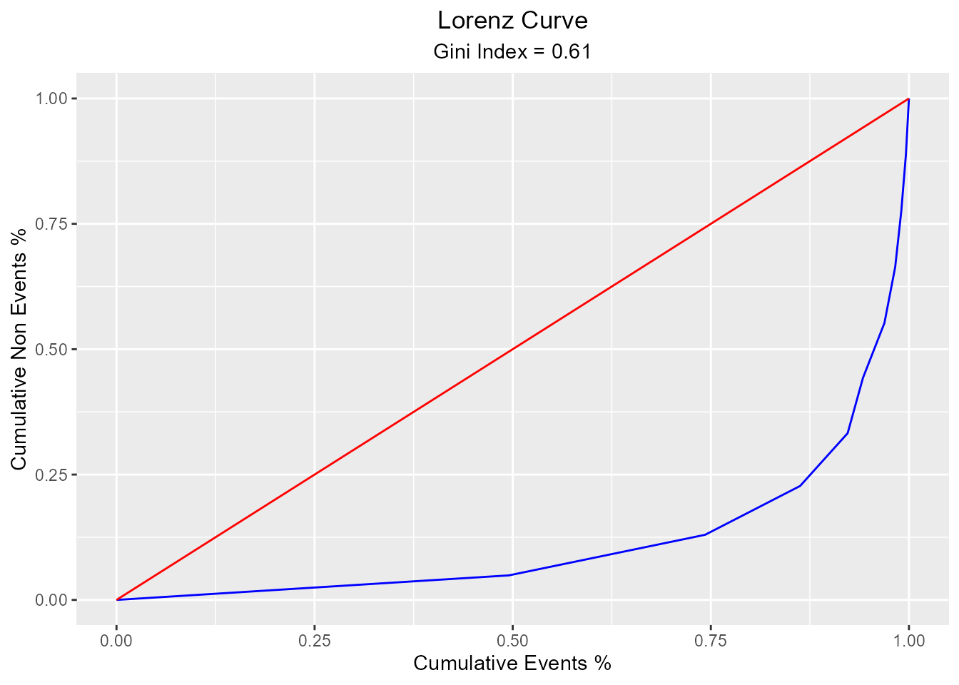
Lorenz Curve
The Lorenz curve is a simple graphic device which illustrates the degree of inequality in the distribution of thevariable concerned. It is a visual representation of inequality used to measure the discriminatory power of the predictive model.
blr_lorenz_curve(model)