Tools for building binary logistic regression models
Overview
Tools designed to make it easier for users, particularly beginner/intermediate R users to build logistic regression models. Includes comprehensive regression output, variable selection procedures, model validation techniques and a ‘shiny’ app for interactive model building.
Installation
# Install blorr from CRAN
install.packages("blorr")

# Install development version from GitHub
# install.packages("devtools")
devtools::install_github("rsquaredacademy/blorr")

# Install the development version from `rsquaredacademy` universe
install.packages("blorr", repos = "https://rsquaredacademy.r-universe.dev")Usage
blorr uses consistent prefix blr_* for easy tab completion.
Bivariate Analysis
blr_bivariate_analysis(hsb2, honcomp, female, prog, race, schtyp)
#>                          Bivariate Analysis
#> ---------------------------------------------------------------------
#> Variable    Information Value    LR Chi Square    LR DF    LR p-value
#> ---------------------------------------------------------------------
#>  female           0.10              3.9350          1        0.0473
#>   prog            0.43              16.1450         2        3e-04
#>   race            0.33              11.3694         3        0.0099
#>  schtyp           0.00              0.0445          1        0.8330
#> ---------------------------------------------------------------------
Weight of Evidence & Information Value
blr_woe_iv(hsb2, prog, honcomp)
#>                            Weight of Evidence
#> -------------------------------------------------------------------------
#> levels    count_0s    count_1s    dist_0s    dist_1s        woe      iv
#> -------------------------------------------------------------------------
#>   1          38          7           0.26       0.13       0.67     0.08
#>   2          65          40          0.44       0.75      -0.53     0.17
#>   3          44          6           0.30       0.11       0.97     0.18
#> -------------------------------------------------------------------------
#>
#>       Information Value
#> -----------------------------
#> Variable    Information Value
#> -----------------------------
#>   prog           0.4329
#> -----------------------------Regression Output
blr_regress(model)
#>                              Model Overview
#> ------------------------------------------------------------------------
#> Data Set    Resp Var    Obs.    Df. Model    Df. Residual    Convergence
#> ------------------------------------------------------------------------
#>   data      honcomp     200        199           196            TRUE
#> ------------------------------------------------------------------------
#>
#>                     Response Summary
#> --------------------------------------------------------
#> Outcome        Frequency        Outcome        Frequency
#> --------------------------------------------------------
#>    0              147              1              53
#> --------------------------------------------------------
#>
#>                   Maximum Likelihood Estimates
#> -----------------------------------------------------------------
#>  Parameter     DF    Estimate    Std. Error    z value    Pr(>|z|)
#> -----------------------------------------------------------------
#> (Intercept)    1     -12.7772       1.9755    -6.4677      0.0000
#>   female1      1      1.4825        0.4474     3.3139       9e-04
#>    read        1      0.1035        0.0258     4.0186       1e-04
#>   science      1      0.0948        0.0305     3.1129      0.0019
#> -----------------------------------------------------------------
#>
#>  Association of Predicted Probabilities and Observed Responses
#> ---------------------------------------------------------------
#> % Concordant          0.8561          Somers' D        0.7147
#> % Discordant          0.1425          Gamma            0.7136
#> % Tied                0.0014          Tau-a            0.2794
#> Pairs                  7791           c                0.8568
#> ---------------------------------------------------------------
Model Fit Statistics
blr_model_fit_stats(model)
#>                               Model Fit Statistics
#> ---------------------------------------------------------------------------------
#> Log-Lik Intercept Only:      -115.644    Log-Lik Full Model:              -80.118
#> Deviance(196):                160.236    LR(3):                            71.052
#>                                          Prob > LR:                         0.000
#> MCFadden's R2                   0.307    McFadden's Adj R2:                 0.273
#> ML (Cox-Snell) R2:              0.299    Cragg-Uhler(Nagelkerke) R2:        0.436
#> McKelvey & Zavoina's R2:        0.518    Efron's R2:                        0.330
#> Count R2:                       0.810    Adj Count R2:                      0.283
#> BIC:                          181.430    AIC:                             168.236
#> ---------------------------------------------------------------------------------
Confusion Matrix
blr_confusion_matrix(model)
#> Confusion Matrix and Statistics
#>
#>           Reference
#> Prediction   0   1
#>          0 135  26
#>          1  12  27
#>
#>
#>                 Accuracy : 0.8100
#>      No Information Rate : 0.7350
#>
#>                    Kappa : 0.4673
#>
#> McNemars's Test P-Value  : 0.0350
#>
#>              Sensitivity : 0.5094
#>              Specificity : 0.9184
#>           Pos Pred Value : 0.6923
#>           Neg Pred Value : 0.8385
#>               Prevalence : 0.2650
#>           Detection Rate : 0.1350
#>     Detection Prevalence : 0.1950
#>        Balanced Accuracy : 0.7139
#>                Precision : 0.6923
#>                   Recall : 0.5094
#>
#>         'Positive' Class : 1
Hosmer Lemeshow Test
blr_test_hosmer_lemeshow(model)
#>            Partition for the Hosmer & Lemeshow Test
#> --------------------------------------------------------------
#>                         def = 1                 def = 0
#> Group    Total    Observed    Expected    Observed    Expected
#> --------------------------------------------------------------
#>   1       20         0          0.16         20        19.84
#>   2       20         0          0.53         20        19.47
#>   3       20         2          0.99         18        19.01
#>   4       20         1          1.64         19        18.36
#>   5       21         3          2.72         18        18.28
#>   6       19         3          4.05         16        14.95
#>   7       20         7          6.50         13        13.50
#>   8       20         10         8.90         10        11.10
#>   9       20         13        11.49         7          8.51
#>  10       20         14        16.02         6          3.98
#> --------------------------------------------------------------
#>
#>      Goodness of Fit Test
#> ------------------------------
#> Chi-Square    DF    Pr > ChiSq
#> ------------------------------
#>   4.4998      8       0.8095
#> ------------------------------
Gains Table
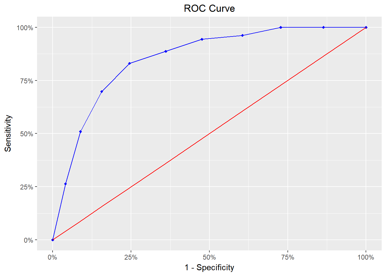
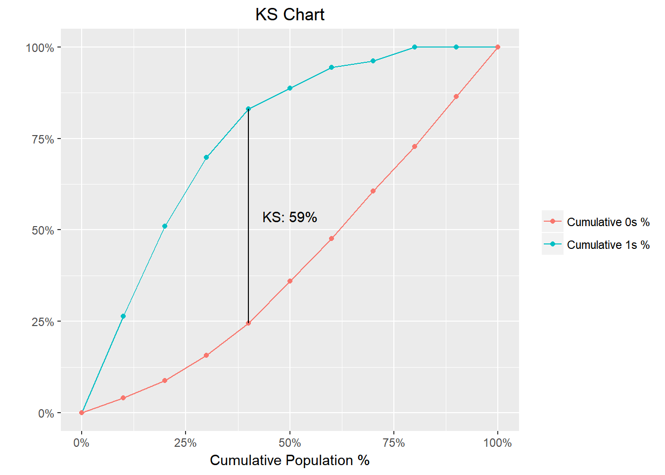
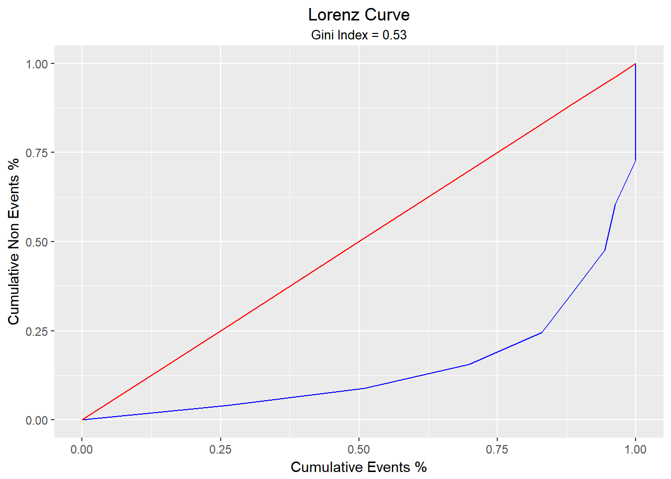
blr_gains_table(model)
#>    decile total  1  0       ks tp  tn  fp fn sensitivity specificity accuracy
#> 1       1    20 14  6 22.33346 14 141   6 39    26.41509    95.91837     77.5
#> 2       2    20 13  7 42.09986 27 134  13 26    50.94340    91.15646     80.5
#> 3       3    20 10 10 54.16506 37 124  23 16    69.81132    84.35374     80.5
#> 4       4    20  7 13 58.52907 44 111  36  9    83.01887    75.51020     77.5
#> 5       5    20  3 17 52.62482 47  94  53  6    88.67925    63.94558     70.5
#> 6       6    20  3 17 46.72058 50  77  70  3    94.33962    52.38095     63.5
#> 7       7    20  1 19 35.68220 51  58  89  2    96.22642    39.45578     54.5
#> 8       8    20  2 18 27.21088 53  40 107  0   100.00000    27.21088     46.5
#> 9       9    20  0 20 13.60544 53  20 127  0   100.00000    13.60544     36.5
#> 10     10    20  0 20  0.00000 53   0 147  0   100.00000     0.00000     26.5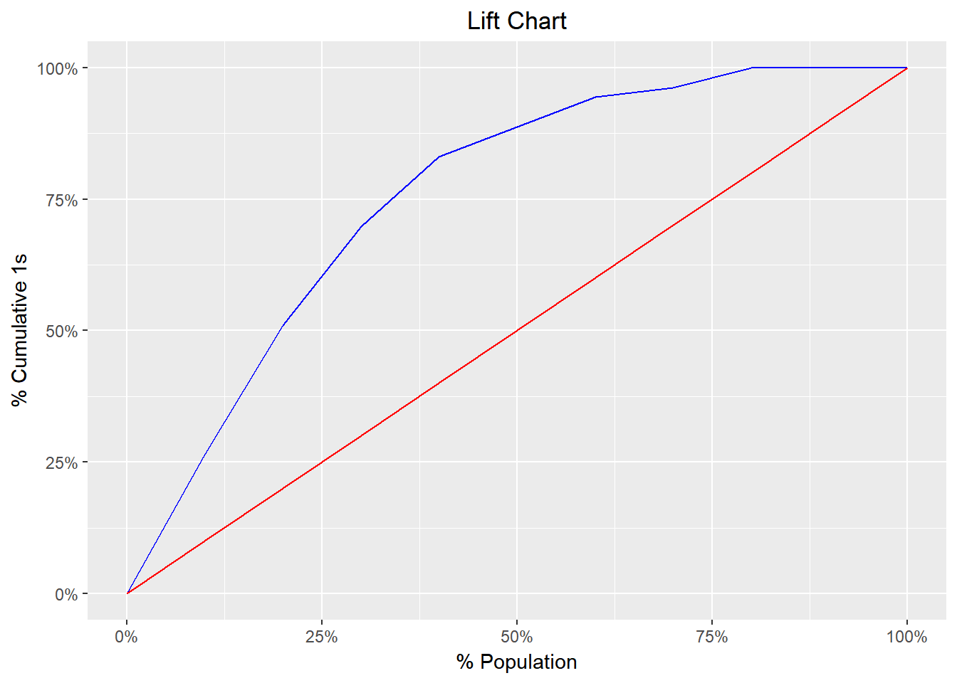
Getting Help
If you encounter a bug, please file a minimal reproducible example using reprex on github. For questions and clarifications, use StackOverflow.
Code of Conduct
Please note that the blorr project is released with a Contributor Code of Conduct. By contributing to this project, you agree to abide by its terms.