Gains table & lift chart

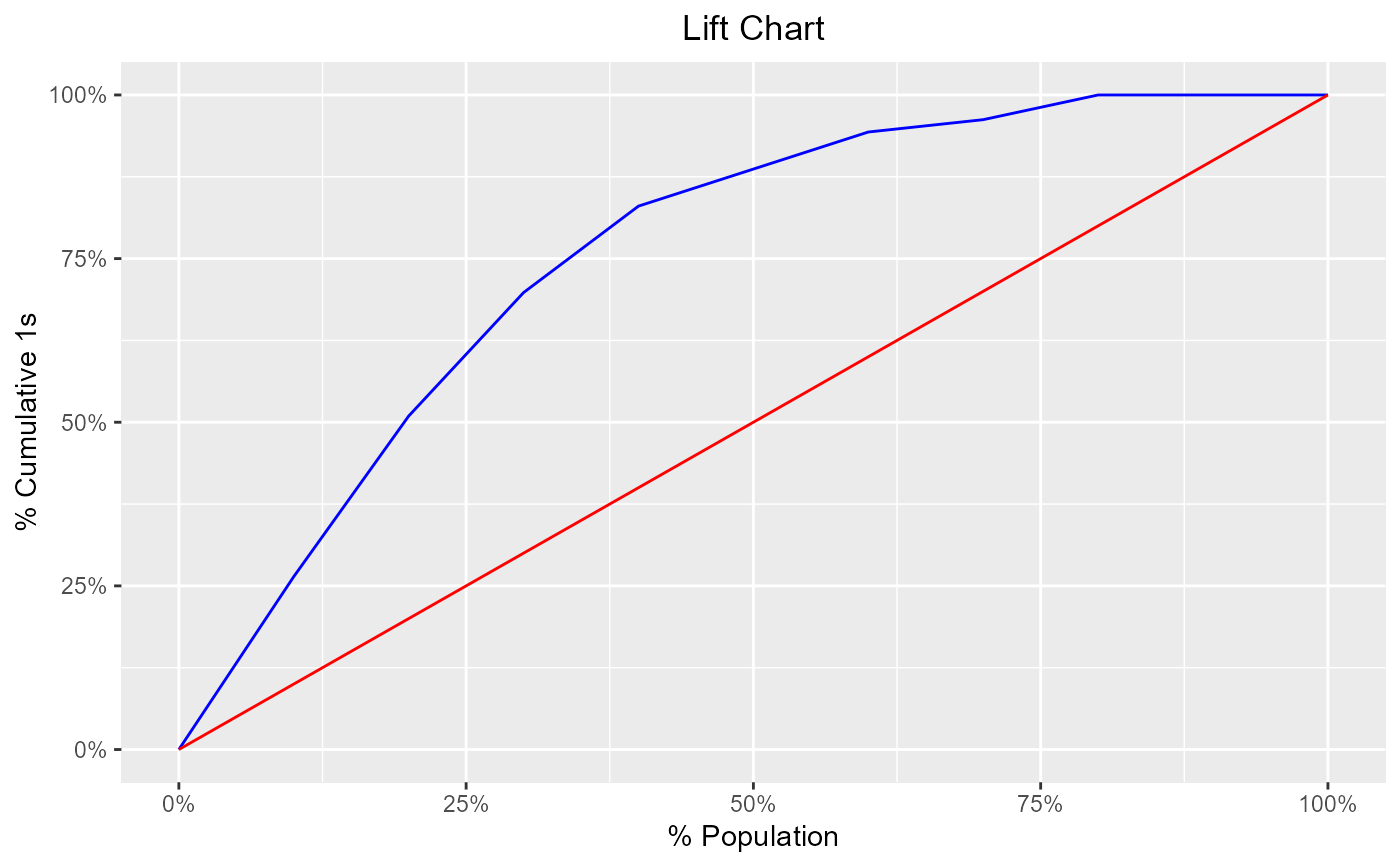
Compute sensitivity, specificity, accuracy and KS statistics to generate the lift chart and the KS chart.

blr_gains_table(model, data = NULL)

# S3 method for blr_gains_table
plot(
  x,
  title = "Lift Chart",
  xaxis_title = "% Population",
  yaxis_title = "% Cumulative 1s",
  diag_line_col = "red",
  lift_curve_col = "blue",
  plot_title_justify = 0.5,
  print_plot = TRUE,
  ...
)

Arguments

model	An object of class glm.
data	A tibble or a data.frame.
x	An object of class blr_gains_table.
title	Plot title.
xaxis_title	X axis title.
yaxis_title	Y axis title.
diag_line_col	Diagonal line color.
lift_curve_col	Color of the lift curve.
plot_title_justify	Horizontal justification on the plot title.
print_plot	logical; if TRUE, prints the plot else returns a plot object.
...	Other inputs.

Value

A tibble.

References

Agresti, A. (2007), An Introduction to Categorical Data Analysis, Second Edition, New York: John Wiley & Sons.

Agresti, A. (2013), Categorical Data Analysis, Third Edition, New York: John Wiley & Sons.

Thomas LC (2009): Consumer Credit Models: Pricing, Profit, and Portfolio. Oxford, Oxford Uni-versity Press.

Sobehart J, Keenan S, Stein R (2000): Benchmarking Quantitative Default Risk Models: A Validation Methodology, Moody’s Investors Service.

See also

Other model validation techniques: blr_confusion_matrix(), blr_decile_capture_rate(), blr_decile_lift_chart(), blr_gini_index(), blr_ks_chart(), blr_lorenz_curve(), blr_roc_curve(), blr_test_hosmer_lemeshow()

Examples

model <- glm(honcomp ~ female + read + science, data = hsb2,
             family = binomial(link = 'logit'))
# gains table
blr_gains_table(model)
#>    decile total  1  0       ks tp  tn  fp fn sensitivity specificity accuracy
#> 1       1    20 14  6 22.33346 14 141   6 39    26.41509    95.91837     77.5
#> 2       2    20 13  7 42.09986 27 134  13 26    50.94340    91.15646     80.5
#> 3       3    20 10 10 54.16506 37 124  23 16    69.81132    84.35374     80.5
#> 4       4    20  7 13 58.52907 44 111  36  9    83.01887    75.51020     77.5
#> 5       5    20  3 17 52.62482 47  94  53  6    88.67925    63.94558     70.5
#> 6       6    20  3 17 46.72058 50  77  70  3    94.33962    52.38095     63.5
#> 7       7    20  1 19 35.68220 51  58  89  2    96.22642    39.45578     54.5
#> 8       8    20  2 18 27.21088 53  40 107  0   100.00000    27.21088     46.5
#> 9       9    20  0 20 13.60544 53  20 127  0   100.00000    13.60544     36.5
#> 10     10    20  0 20  0.00000 53   0 147  0   100.00000     0.00000     26.5

# lift chart
k <- blr_gains_table(model)
plot(k)