library(blorr)
library(magrittr)

Regression Model

model <- glm(y ~ job + housing + contact + poutcome + duration + month +
             campaign + loan + marital + education + day + balance + previous, 
             data = bank_marketing, family = binomial(link = 'logit'))

Confusion Matrix

blr_confusion_matrix(model, cutoff = 0.5)
#> Confusion Matrix and Statistics
#> 
#>           Reference
#> Prediction    0    1
#>          0 3909  339
#>          1   95  178
#>                                          
#>                Accuracy : 0.904          
#>                  95% CI : (0.895, 0.9124)
#>     No Information Rate : 0.8856         
#>     P-Value [Acc > NIR] : 3.984e-05      
#>                                          
#>                   Kappa : 0.4035         
#>  Mcnemar's Test P-Value : < 2.2e-16      
#>                                          
#>             Sensitivity : 0.34429        
#>             Specificity : 0.97627        
#>          Pos Pred Value : 0.65201        
#>          Neg Pred Value : 0.92020        
#>              Prevalence : 0.11436        
#>          Detection Rate : 0.03937        
#>    Detection Prevalence : 0.06038        
#>       Balanced Accuracy : 0.66028        
#>                                          
#>        'Positive' Class : 1              
#> 

Hosmer Lemeshow Test

blr_test_hosmer_lemeshow(model)
#>            Partition for the Hosmer & Lemeshow Test            
#> --------------------------------------------------------------
#>                         def = 1                 def = 0        
#> Group    Total    Observed    Expected    Observed    Expected 
#> --------------------------------------------------------------
#>   1       453        0          2.14        453        450.86  
#>   2       452        2          4.72        450        447.28  
#>   3       452        3          7.77        449        444.23  
#>   4       452        2         11.32        450        440.68  
#>   5       452        11        15.72        441        436.28  
#>   6       452        13        21.46        439        430.54  
#>   7       452        30        30.56        422        421.44  
#>   8       452        47        49.64        405        402.36  
#>   9       452       141        97.93        311        354.07  
#>  10       452       268        275.74       184        176.26  
#> --------------------------------------------------------------
#> 
#>      Goodness of Fit Test      
#> ------------------------------
#> Chi-Square    DF    Pr > ChiSq 
#> ------------------------------
#>  44.4637      8       0.0000   
#> ------------------------------

Gains Table

blr_gains_table(model)
#> # A tibble: 10 x 12
#>    decile total   `1`   `0`    ks    tp    tn    fp    fn sensitivity
#>     <dbl> <int> <int> <int> <dbl> <int> <int> <int> <int>       <dbl>
#>  1   1.00   452   268   184  47.2   268  3820   184   249        51.8
#>  2   2.00   452   141   311  66.7   409  3509   495   108        79.1
#>  3   3.00   452    47   405  65.7   456  3104   900    61        88.2
#>  4   4.00   452    30   422  61.0   486  2682  1322    31        94.0
#>  5   5.00   452    13   439  52.5   499  2243  1761    18        96.5
#>  6   6.00   452    11   441  43.7   510  1802  2202     7        98.6
#>  7   7.00   452     2   450  32.8   512  1352  2652     5        99.0
#>  8   8.00   452     3   449  22.2   515   903  3101     2        99.6
#>  9   9.00   452     2   450  11.3   517   453  3551     0       100  
#> 10  10.0    453     0   453   0     517     0  4004     0       100  
#> # ... with 2 more variables: specificity <dbl>, accuracy <dbl>

Lift Chart

model %>%
    blr_gains_table() %>%
    plot()

ROC Curve

model %>%
    blr_gains_table() %>%
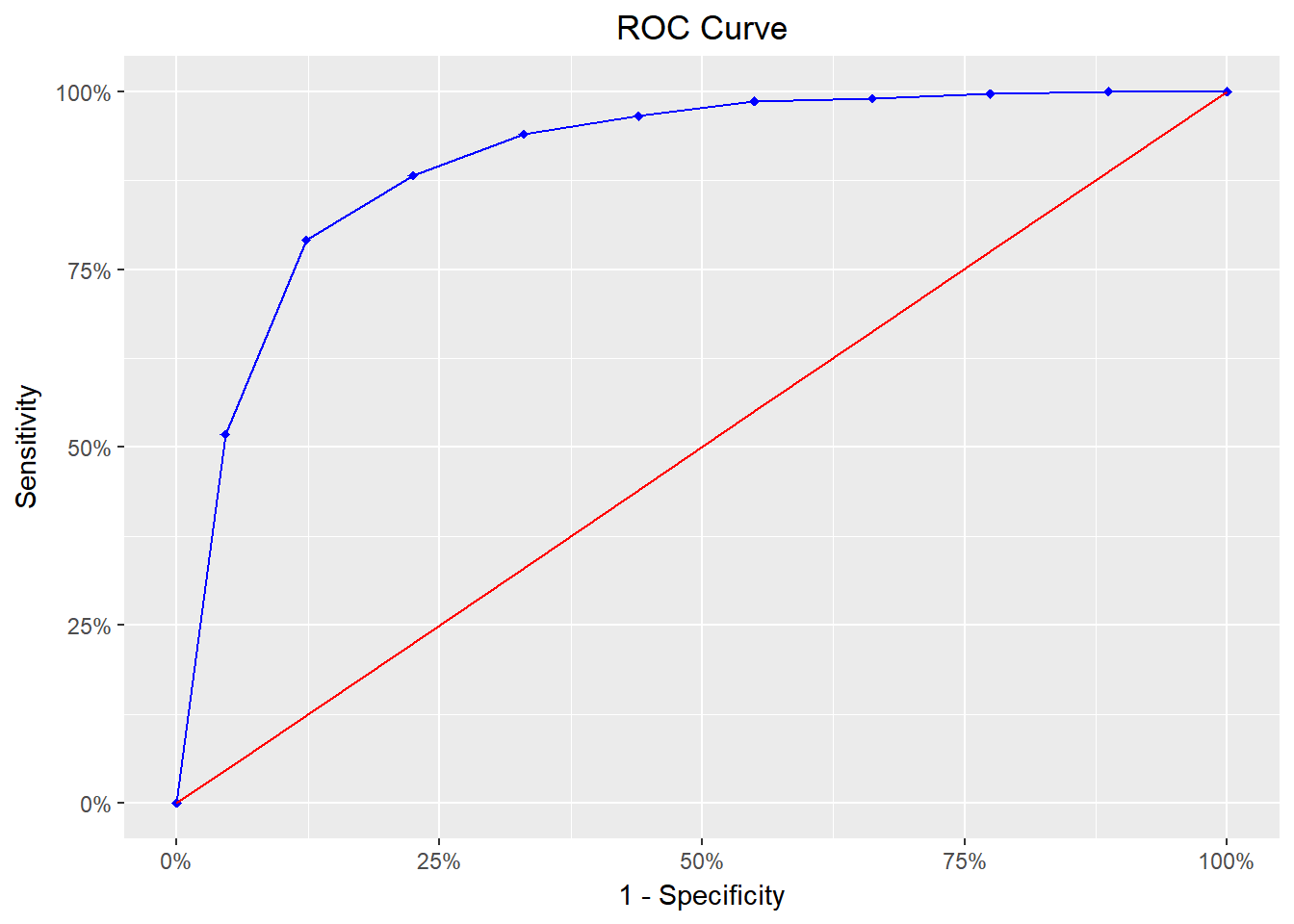
  blr_roc_curve()

KS Chart

model %>%
    blr_gains_table() %>%
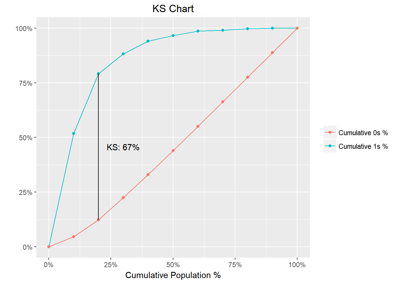
  blr_ks_chart()

Decile Lift Chart

model %>%
  blr_gains_table() %>%
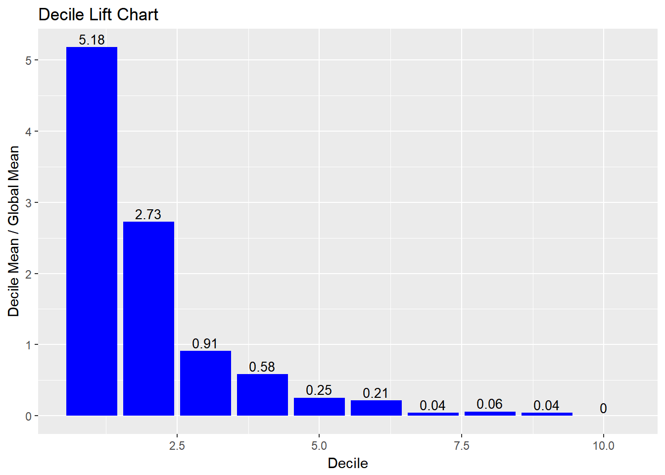
  blr_decile_lift_chart()

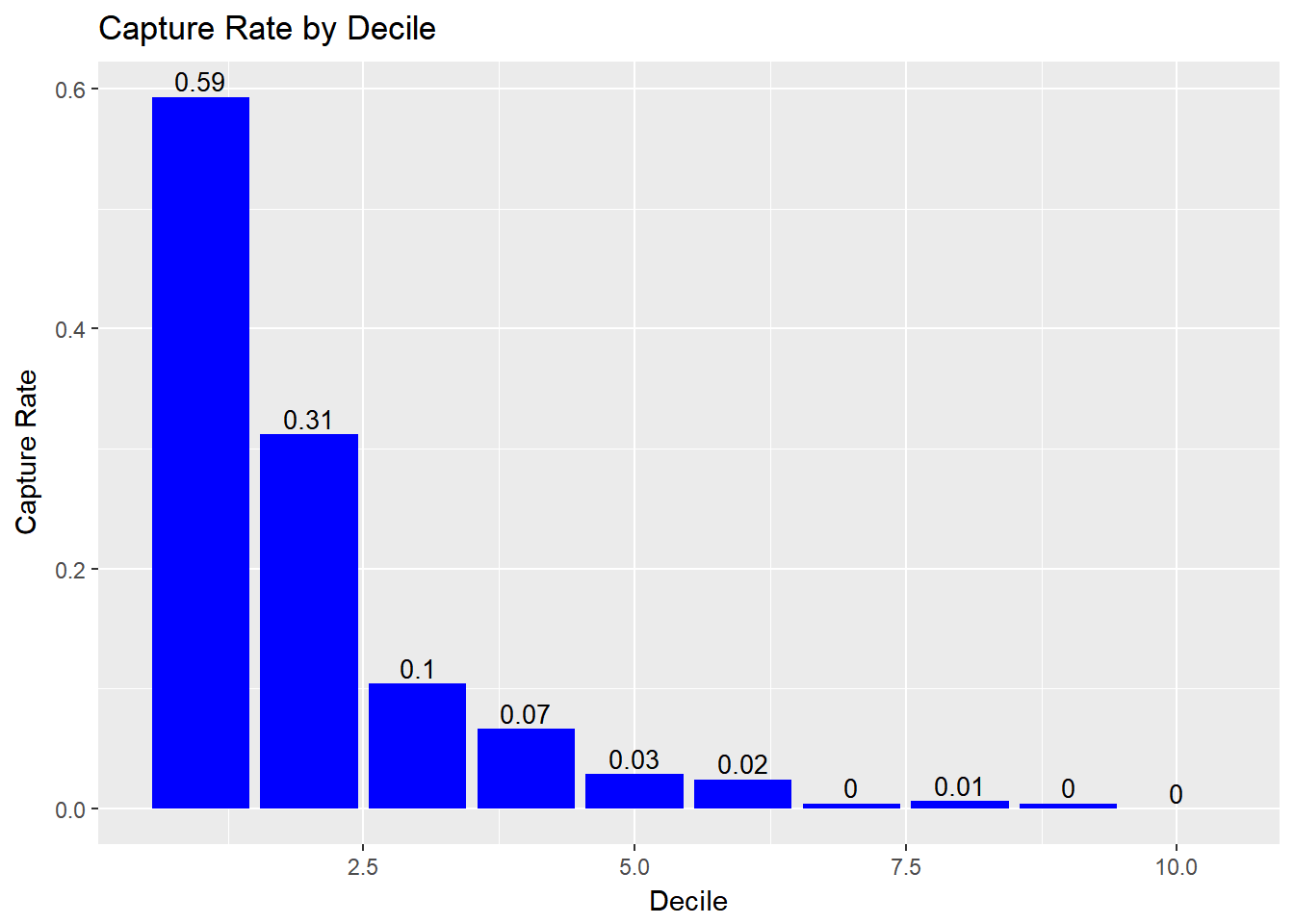
Capture Rate by Decile

model %>%
  blr_gains_table() %>%
  blr_decile_capture_rate()

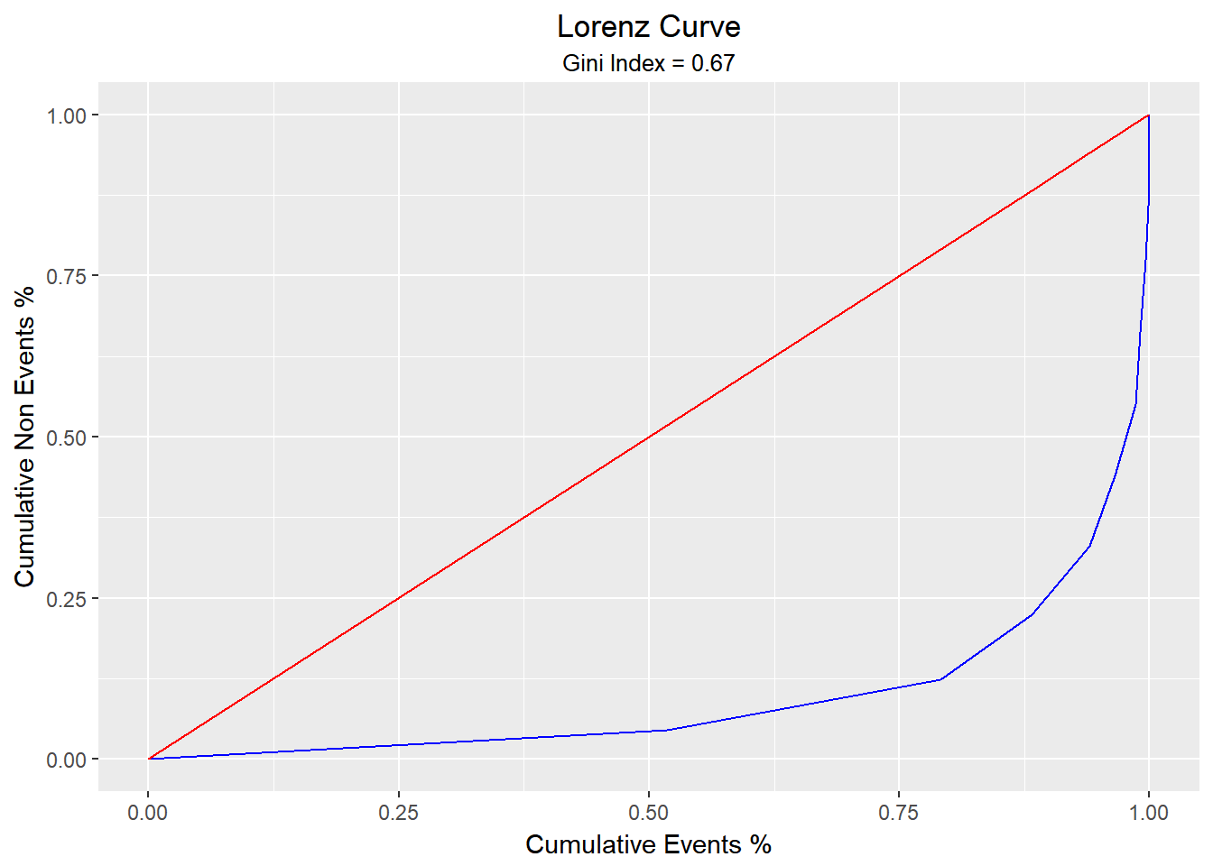
Lorenz Curve

blr_lorenz_curve(model)